半参数回归模型
[原创]
常见的处理非线性关系的方法有数据转换方法和神经转换、SVM、投影寻踪和基于树的方法等高计算强度方法。实际在应用回归问题有很大的局限性,模型的可解释性差。使用非参数和半参数回归方法来处理非线性关系一定程度可避免这些问题。
从数据本身出发来估计适合数据本身的函数形式。
- 1.忽略非线性的后果
对模型所有的连续自变量都进行检验来判断是否具有非线性作用(xy),通过数据变换解决非线性问题。
- 2.数据变换
幂转换:仅能够对正数取值的变量才能使用。所以才使用非参数和半参数回归方法。
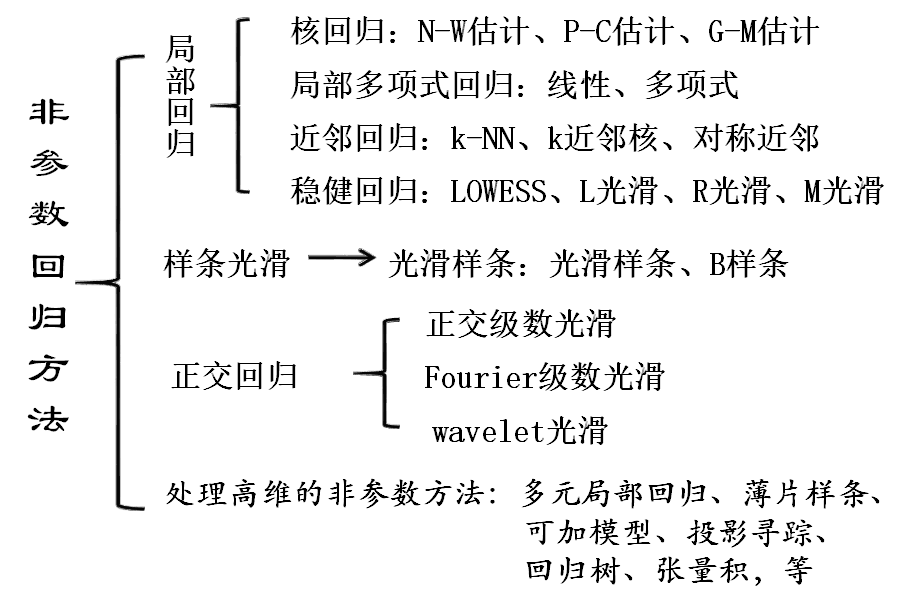
- 3.非参数和半参数回归方法
- 从数据本身出发来估计适合数据本身的函数形式。用局部估计取代全局估计。
- 非参数回归的局部估计是通过数据估计两个变量之间的函数形式,而全局估计通过假设来对函数形式作出规定。
- 半参数回归模型:利用多元模型把全局估计和局部估计结合起来。
- 半参数回归模型:广义可加模型(GAM)(特殊:加性模型)。
- GAM指自变量为离散或连续变量的半参数回归模型,可对自变量做非参数估计,对一些自变量采取标准的方式估计。
- GAM中怀疑具有非线性函数形式的连续自变量可以用非参数估计,而模型中其他变量仍以参数形式估计。
- GAM依赖非参数回归,X与Y之间的全局拟合被局部拟合取代,放弃了全部拟合的假设,仍保留了加性的假设。
- GAM的加性假设使得模型比神经网络、支持向量机等更容易解释,比完全的参数模型更灵活。
- GAM可以适用于许多类型的因变量:连续的、计数的、二分类的,定序的和时间等等。
- GAM提供了诊断非线性的框架,简单线性模型和幂转换模型是嵌套在GAM中。
- GAM的局部估计可以使用F检验或似然比检验来检验线性,二次项或任何其他幂转换模型的拟合效果。如果半参数回归模型优于线性模型或幂转换模型,它就应该被采用。
- 半参数回归模型的检验非线性和模型比较作用给予了半参数回归模型的强大功能,对于任意的连续自变量,都应采用半参数方法进行诊断或建模。
1 非参数估计
参数回归与非参数回归的优缺点比较
> 参数模型
>
> 优点:
> (1)模型形式简单明确,仅由一些参数表达
> (2)在经济中,模型的参数具有一般都具有明确的经济含义
> (3)当模型参数假设成立,统计推断的精度较高,能经受实际检验
> (4)模型能够进行外推运算
> (5)模型可以用于小样本的统计推断
>
> 缺点:
> (1)回归函数的形式预先假定
> (2)模型限制较多:一般要求样本满足某种分布要求,随机误差满足正态假设,解释变量间独立,解释变量与随机误差不相关等
> (3)需要对模型的参数进行严格的检验推断,步骤较多
> (4)模型泛化能力弱,缺乏稳健性,当模型假设不成立,拟合效果不好,需要修正或者甚至更换模型
>
> 非参数模型
>
> 优点:
>
> (1)**回归函数形式自由,受约束少,对数据的分布一般不做任何要求**
> (2)**适应能力强,稳健性高,回归模型完全由数据驱动**
> (3)**模型的精度高 ;**
> (4)**对于非线性、非齐次问题,有非常好的效果**
使用非参数回归时,利用数据来估计F的函数形式。 事先的线性假设被更弱的假设光滑总体函数所代替。这个更弱的假设的代价是两方面的: * 第一,计算方面的代价是巨大的,但考虑到现代计算技术的速度,这不再是大问题; * 第二,失去了一些可解释性,但同时也得到了一个更具代表性的估计。
光滑的定义:函数在所有点处的一阶导数都存在。
2 半参数估计
对于非参数估计来说,当自变量个数超过2个的情况,非参数回归就难以应用。
如果假设自变量对因变量的作用是可加的,那么就可以得到一个部分自变量以参数形式进入而另一部分自变量以非参数形式进入的半参数回归模型。
半参数回归模型可以在熟悉的多元回归模型背景下估计带有非线性估计的标准参数模型,非参数项可以用于连续自变量或用于非线性的检验。
1 可加模型和半参数模型
1.1 多元非参数回归
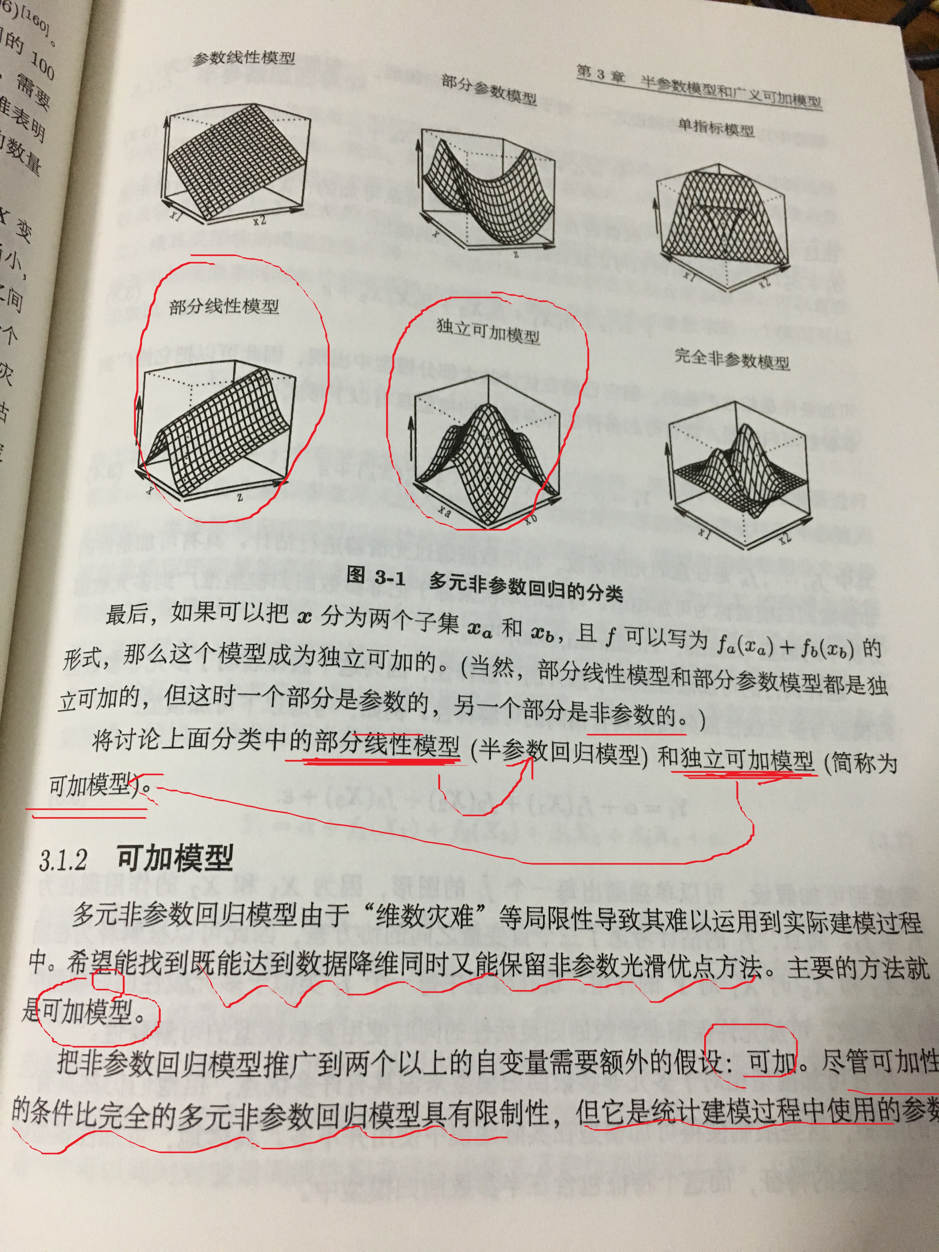
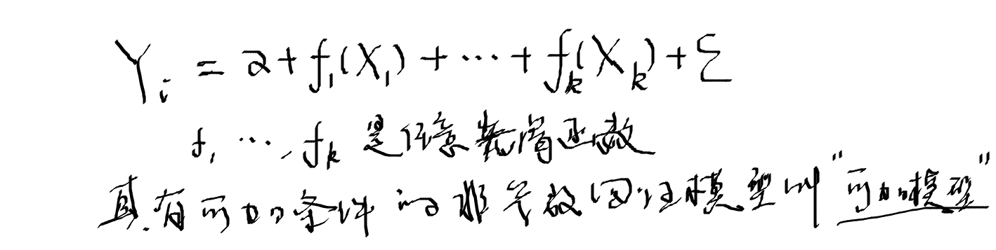
1.2 可加模型
1.3 半参数回归模型
如果只估计连续变量之间的非线性关系,可加模型刚好合适,但是实际建模中并不都是非线性关系。
离散自变量是非常普遍的,而且个数通常比连续自变量个数多;
有的自变量与因变量之间可能是线性关系;
如果一个参数足够描述X与Y之间的关系,就没有必要使用额外的参数来估计非参数回归;
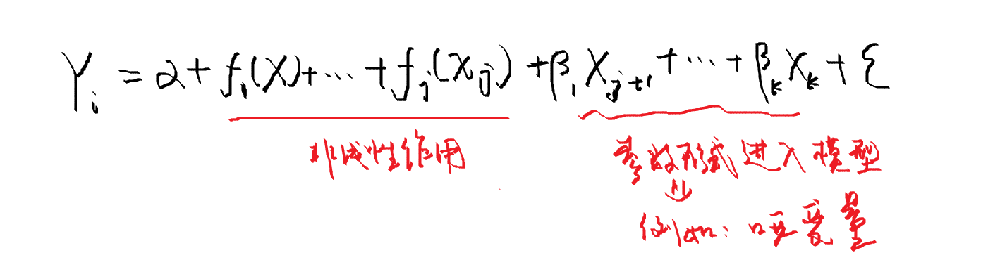
最具灵活性的模型应该是同一个模型中既含有参数项又包含非参数项。
可以直接修改可加模型来同时估计参数项和非参数项,混合参数项和非参数项的一个模型采取以下形式:
最精彩的部分:
半参数回归模型可以估计种类非常多的函数形式,模型中的参数部分允许像哑变量或定序变量的离散变量与非参数项一起建模。
对Y的作用为线性的连续自变量可以以参数方式进行估计以节省参数。
半参数模型相对于完全的参数模型也具有优势,非参数的推断在半参数回归模型中得到了保留,它允许检验任何一个非参数项对于模型来说是否需要。
半参数模型还可以在半参数光滑模型中包含交互项。
2 广义线性模型(GLM)
实际数据分析中,分类数据非常广泛。统计上,分类数据的模型一般属于广义线性模型(GLM)。
把半参数回归模型推广到分类数据等情形,需要与广义线性模型类似的框架,才能得到广义可加线性模型(GAM)。
经典的线性模型的假设:
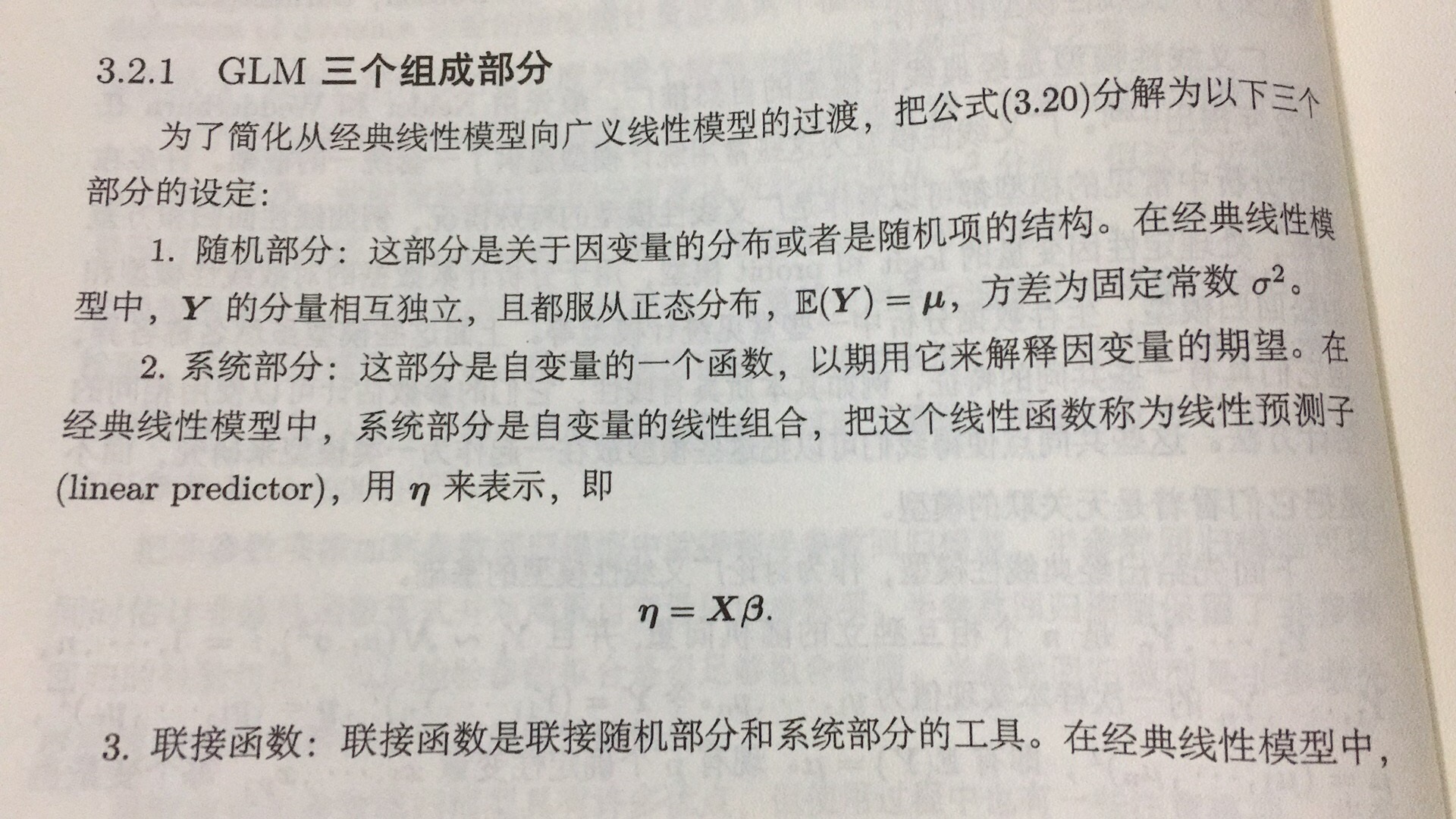
(1)线性,即因变量的期望是自变量参数的线性函数;
(2)独立性,Y1,…,Yn之间是独立的;
(3)正态性,Y1,…,Yn都服从正态分布;
(4)方差齐性,Y1,…,Yn的方差为固定常数;
3 广义可加模型(GAM)
4 GAM模型实操
pyGAM是一个用于在Python中构建“广义可加模型”的包,重点是模块化和性能。 任何具有scikit-learn或scipy经验的人都会立即熟悉API。
更多内容请参考以下地址:
https://pygam.readthedocs.io/en/latest/
https://multithreaded.stitchfix.com/blog/2015/07/30/gam/
1 安装
pip install pygam
为了加速对具有约束的大型模型进行优化,安装scikit-sparse会有所帮助,因为它包含一个稍快,稀疏版本的Cholesky分解。 从scikit-sparse导入。
2.建模
In [1]: from pygam.datasets import wage

In [2]: X, y = wage()

In [3]: from pygam import LinearGAM, s, f

In [4]: gam = LinearGAM(s(0) + s(1) + f(2)).fit(X, y)

In [5]: gam.summary()
LinearGAM
=============================================== ==========================================================
Distribution:                        NormalDist Effective DoF:                                     25.1911
Link Function:                     IdentityLink Log Likelihood:                                -24118.6847
Number of Samples:                         3000 AIC:                                            48289.7516
                                                AICc:                                           48290.2307
                                                GCV:                                             1255.6902
                                                Scale:                                           1236.7251
                                                Pseudo R-Squared:                                   0.2955
==========================================================================================================
Feature Function                  Lambda               Rank         EDoF         P > x        Sig. Code
================================= ==================== ============ ============ ============ ============
s(0)                              [0.6]                20           7.1          5.95e-03     **
s(1)                              [0.6]                20           14.1         1.11e-16     ***
f(2)                              [0.6]                5            4.0          1.11e-16     ***
intercept                                              1            0.0          1.11e-16     ***
==========================================================================================================
Significance codes:  0 '***' 0.001 '**' 0.01 '*' 0.05 '.' 0.1 ' ' 1

WARNING: Fitting splines and a linear function to a feature introduces a model identifiability problem
         which can cause p-values to appear significant when they are not.

WARNING: p-values calculated in this manner behave correctly for un-penalized models or models with
         known smoothing parameters, but when smoothing parameters have been estimated, the p-values
         are typically lower than they should be, meaning that the tests reject the null too readily.
C:\Anaconda3\Scripts\ipython:1: UserWarning: KNOWN BUG: p-values computed in this summary are likely much smaller than they should be.

Please do not make inferences based on these values!

Collaborate on a solution, and stay up to date at:
github.com/dswah/pyGAM/issues/163
即使我们有3个项,总共(20 + 20 + 5)= 45个自由变量,默认的平滑罚分(lam = 0.6)会将Effective DoF-有效自由度降低到~25。
默认情况下,样条曲线s(…)使用20个基函数。 这是一个很好的起点。 经验法则是使用相当大的灵活性,然后让平滑罚分使模型正规化。
但是,我们始终可以使用我们的专业知识在需要的地方增加灵活性,或删除基本功能,并使拟合更容易:
In [6]: gam = LinearGAM(s(0, n_splines=5) + s(1) + f(2)).fit(X, y)

In [7]: gam.summary()
LinearGAM
=============================================== ==========================================================
Distribution:                        NormalDist Effective DoF:                                       22.26
Link Function:                     IdentityLink Log Likelihood:                                -24118.7429
Number of Samples:                         3000 AIC:                                             48284.006
                                                AICc:                                           48284.3852
                                                GCV:                                              1253.479
                                                Scale:                                           1236.7487
                                                Pseudo R-Squared:                                   0.2948
==========================================================================================================
Feature Function                  Lambda               Rank         EDoF         P > x        Sig. Code
================================= ==================== ============ ============ ============ ============
s(0)                              [0.6]                5            4.1          4.22e-03     **
s(1)                              [0.6]                20           14.2         1.11e-16     ***
f(2)                              [0.6]                5            4.0          1.11e-16     ***
intercept                                              1            0.0          1.11e-16     ***
==========================================================================================================
Significance codes:  0 '***' 0.001 '**' 0.01 '*' 0.05 '.' 0.1 ' ' 1

WARNING: Fitting splines and a linear function to a feature introduces a model identifiability problem
         which can cause p-values to appear significant when they are not.

WARNING: p-values calculated in this manner behave correctly for un-penalized models or models with
         known smoothing parameters, but when smoothing parameters have been estimated, the p-values
         are typically lower than they should be, meaning that the tests reject the null too readily.
C:\Anaconda3\Scripts\ipython:1: UserWarning: KNOWN BUG: p-values computed in this summary are likely much smaller than they should be.

Please do not make inferences based on these values!

Collaborate on a solution, and stay up to date at:
github.com/dswah/pyGAM/issues/163
3.模型自动调参
默认情况下,样条项,s()对它们的二阶导数有一个惩罚,这会使函数更平滑,而因子项f()和线性项l()有一个l2,即岭惩罚,它会使它们采取较小的值。
lam,λ的缩写,控制每个项的正则化惩罚的强度。 样条项、因子项和线性项可以有多个处罚,因此多个lam。
In [8]: print(gam.lam)
[[0.6], [0.6], [0.6]]
我们的模型有3个参数,目前每个项只有一个。
让我们对多个lam值执行网格搜索,看看我们是否可以改进我们的模型。
我们将寻找具有最低广义交叉验证(GCV)分数的模型。
我们的搜索空间是三维的,因此我们必须保持每个维度考虑的点数。
让我们为每个平滑参数尝试5个值,结果在我们的网格中总共有5 * 5 * 5 = 125个点。
In [9]: import numpy as np
   ...:
   ...: lam = np.logspace(-3, 5, 5)
   ...: lams = [lam] * 3
   ...:
   ...: gam.gridsearch(X, y, lam=lams)
   ...: gam.summary()
   ...:
   ...:
100% (125 of 125) |####################################################################################################| Elapsed Time: 0:00:19 Time:  0:00:19
LinearGAM
=============================================== ==========================================================
Distribution:                        NormalDist Effective DoF:                                      9.2948
Link Function:                     IdentityLink Log Likelihood:                                -24119.7277
Number of Samples:                         3000 AIC:                                            48260.0451
                                                AICc:                                           48260.1229
                                                GCV:                                              1244.089
                                                Scale:                                           1237.1528
                                                Pseudo R-Squared:                                   0.2915
==========================================================================================================
Feature Function                  Lambda               Rank         EDoF         P > x        Sig. Code
================================= ==================== ============ ============ ============ ============
s(0)                              [100000.]            5            2.0          7.54e-03     **
s(1)                              [1000.]              20           3.3          1.11e-16     ***
f(2)                              [0.1]                5            4.0          1.11e-16     ***
intercept                                              1            0.0          1.11e-16     ***
==========================================================================================================
Significance codes:  0 '***' 0.001 '**' 0.01 '*' 0.05 '.' 0.1 ' ' 1

WARNING: Fitting splines and a linear function to a feature introduces a model identifiability problem
         which can cause p-values to appear significant when they are not.

WARNING: p-values calculated in this manner behave correctly for un-penalized models or models with
         known smoothing parameters, but when smoothing parameters have been estimated, the p-values
         are typically lower than they should be, meaning that the tests reject the null too readily.
C:\Anaconda3\Scripts\ipython:7: UserWarning: KNOWN BUG: p-values computed in this summary are likely much smaller than they should be.

Please do not make inferences based on these values!

Collaborate on a solution, and stay up to date at:
github.com/dswah/pyGAM/issues/163
这要好一点。 即使样本内的R2值较低,我们也可以期望我们的模型更好地推广,因为GCV误差较低。
通过使用训练/测试分割,并在测试集上检查模型的错误,我们可以更严格。 我们也非常懒,只在我们的hyperopt中尝试了125个值。 如果我们花更多时间在更多点上搜索,我们可能会找到更好的模型。
对于高维搜索空间,尝试随机搜索有时是个好主意。
我们可以通过使用numpy的random模块来实现这一点:
In [10]: lams = np.random.rand(100, 3) # random points on [0, 1], with shape (100, 3)
    ...: lams = lams * 8 - 3 # shift values to -3, 3
    ...: lams = np.exp(lams) # transforms values to 1e-3, 1e3

In [11]: random_gam =  LinearGAM(s(0) + s(1) + f(2)).gridsearch(X, y, lam=lams)
    ...: random_gam.summary()
100% (100 of 100) |####################################################################################################| Elapsed Time: 0:00:20 Time:  0:00:20
LinearGAM
=============================================== ==========================================================
Distribution:                        NormalDist Effective DoF:                                     15.7892
Link Function:                     IdentityLink Log Likelihood:                                -24115.5854
Number of Samples:                         3000 AIC:                                            48264.7493
                                                AICc:                                           48264.9496
                                                GCV:                                             1247.2565
                                                Scale:                                           1235.4461
                                                Pseudo R-Squared:                                    0.294
==========================================================================================================
Feature Function                  Lambda               Rank         EDoF         P > x        Sig. Code
================================= ==================== ============ ============ ============ ============
s(0)                              [146.5848]           20           6.3          6.98e-03     **
s(1)                              [113.6698]           20           5.6          1.11e-16     ***
f(2)                              [0.0907]             5            4.0          1.11e-16     ***
intercept                                              1            0.0          1.11e-16     ***
==========================================================================================================
Significance codes:  0 '***' 0.001 '**' 0.01 '*' 0.05 '.' 0.1 ' ' 1

WARNING: Fitting splines and a linear function to a feature introduces a model identifiability problem
         which can cause p-values to appear significant when they are not.

WARNING: p-values calculated in this manner behave correctly for un-penalized models or models with
         known smoothing parameters, but when smoothing parameters have been estimated, the p-values
         are typically lower than they should be, meaning that the tests reject the null too readily.
C:\Anaconda3\Scripts\ipython:2: UserWarning: KNOWN BUG: p-values computed in this summary are likely much smaller than they should be.

Please do not make inferences based on these values!

Collaborate on a solution, and stay up to date at:
github.com/dswah/pyGAM/issues/163
- 在这种情况下,我们的确定性搜索找到了更好的模型:
In [12]: gam.statistics_['GCV'] < random_gam.statistics_['GCV']

Out[12]: True
在安装模型后填充统计信息属性。 有许多有趣的模型统计信息需要检查,尽管许多都会在模型摘要中自动报告:
In [13]: list(gam.statistics_.keys())
Out[13]:
['UBRE',
 'edof',
 'scale',
 'AIC',
 'pseudo_r2',
 'deviance',
 'loglikelihood',
 'p_values',
 'm_features',
 'GCV',
 'n_samples',
 'AICc',
 'cov',
 'se',
 'edof_per_coef']
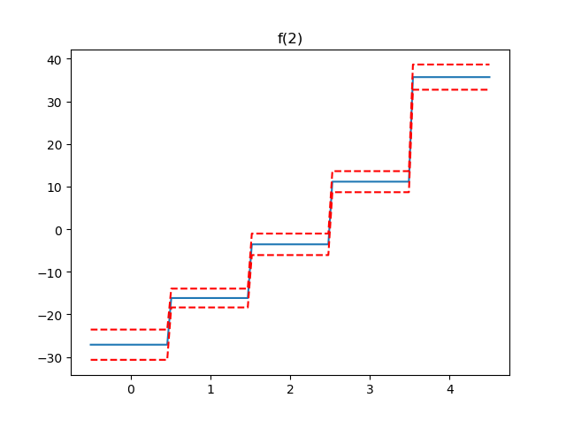
3.部分依赖函数
GAM最吸引人的特性之一是我们可以分解和检查每个特征对整体预测的贡献。
这是通过部分依赖函数完成的。
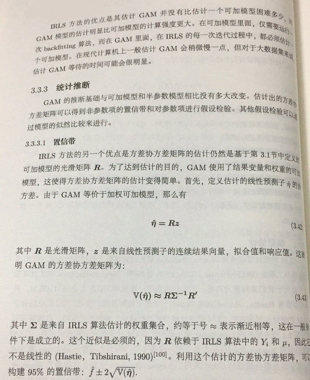
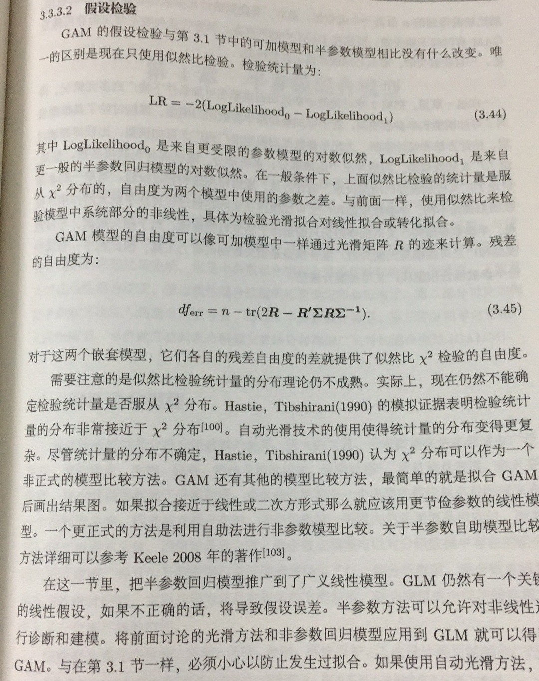
让我们绘制模型中每个项的部分依赖性,以及估计函数的95%置信区间。
In [14]: import matplotlib.pyplot as plt

In [15]: for i, term in enumerate(gam.terms):
    ...:     if term.isintercept:
    ...:         continue
    ...:
    ...:     XX = gam.generate_X_grid(term=i)
    ...:     pdep, confi = gam.partial_dependence(term=i, X=XX, width=0.95)
    ...:
    ...:     plt.figure()
    ...:     plt.plot(XX[:, term.feature], pdep)
    ...:     plt.plot(XX[:, term.feature], confi, c='r', ls='--')
    ...:     plt.title(repr(term))
    ...:     plt.show()
注意:我们跳过截距,因为它没有任何有趣的绘图。